NYISO System & Resource Outlook – Renewable Profiles and Variability

The New York Independent System Operator recently released the 2023-2042 System & Resource Outlook (“Outlook”).  It examines “a wide range of potential future system conditions and compares possible pathways to an increasingly greener resource mix.”  This post summarizes the key findings of Appendix E: New York Renewable Profiles and Variability.

I have followed the Climate Act since it was first proposed, submitted comments on the Climate Act implementation plan, and have written over 400 articles about New York’s net-zero transition.  The opinions expressed in this article do not reflect the position of any of my previous employers or any other organization have been associated with, these comments are mine alone.

Overview

The Climate Act established a New York “Net Zero” target (85% reduction in GHG emissions and 15% offset of emissions) by 2050.  It includes an interim 2030 reduction target of a 40% GHG reduction by 2030, a 70% electric system renewable energy  mandate by 2030, and a requirement that all electricity generated be “zero-emissions” resources by 2040. The Climate Action Council (CAC) was responsible for preparing the Scoping Plan that outlined how to “achieve the State’s bold clean energy and climate agenda.” The Integration Analysis prepared by the New York State Energy Research and Development Authority (NYSERDA) and its consultants quantifies the impact of the electrification strategies used to reduce greenhouse gas emissions.  That material was used to develop the Draft Scoping Plan outline of strategies.  After a year-long review, the Scoping Plan was finalized at the end of 2022.  Since then, the State has been trying to implement the Scoping Plan recommendations through regulations, Public Service Commission orders, and legislation.

Overview of the Outlook Report

I provided an overview of the NYISO 2023-2042 System & Resource Outlook earlier.  The document and 11 appendices are available at the NYISO website:

• 2023-2042 Outlook Report
• Appendix A – Production Cost Model Benchmark
• Appendix B – Production Cost Assumptions Matrix
• Appendix C – Capacity Expansion Assumptions Matrix
• Appendix D – Modeling & Methodologies
• Appendix E – Renewable Profiles & Variability
• Appendix F – Dispatchable Emission-Free Resources
• Appendix G – Production Cost Model Results
• Appendix H – Capacity Expansion Model Results
• Appendix I – Transmission Congestion Analysis
• Appendix J – Renewable Generation Pockets
• Appendix K – Capacity Expansion Model Sensitivities

The Executive Summary explains that:

• The Outlook examines a wide range of potential future system conditions and compares possible pathways to an increasingly greener resource mix. By simulating several possible future system configurations and forecasting the transmission constraints for each, the NYISO:
• Postulates possible resource mixes that achieve New York’s public policy mandates, while maintaining reserve margins, and capacity requirements;
• Identifies regions of New York where renewable or other resources may be unable to generate at their full capability due to transmission constraints;
• Quantifies the extent to which these transmission constraints limit delivery of renewable energy to consumers; and
• Highlights potential opportunities for transmission investment that may provide economic, policy, and/or operational benefits.

Renewable Resource Characterization

The information presented in Appendix E was developed by DNV.  They modeled “long-term hourly simulated weather and generation profiles for representative offshore wind (OSW), land-based wind (LBW), and utility- scale solar (UPV) generators” in two phases.  Initially DNV assessed the OSW production for seven locations.   In the second phase, the analyzed LBW and UPV generation for nearly 80 LBW and UPV locations each throughout the state.  The projections were used to “determine the zonal or county aggregate net capacity factor (NCF) profiles that the NYISO used as inputs for this Outlook.

The goal of this work is to estimate the energy production of LBW, OSW, and solar—both UPV and behind the meter (BTM) PV.  The report explains:

The production amounts of each type of generation are considered when determining the representative days selected for the capacity expansion model and are used as hourly generation shapes in the production cost model for this Outlook.  The NYISO acknowledges that advances in renewable energy technology are continuously occurring and can lead to improved performance among generators built in the later years of the study period. Offsetting this effect, however, is that better sites may be utilized before less favorable resource sites leading to older technology on more favorable sites. Moreover, once installed, equipment performance can degrade over time. While these impacts are known, the exact magnitude of the impacts is difficult to quantify. Accordingly, this Outlook does not make any assumptions about improved performance of renewable generators built in the later years of the study period or performance degradation of resources once in operation.

The NCF data can be combined with hypothetical wind and solar projects sited throughout the state and in the New York Bight on the Outer Continental Shelf to estimate the generation production that represents actual historical weather conditions.  As the report notes: “The increasing weather dependent supply resources and electrified load will necessitate more attention be paid to the modeling of spatiotemporally correlated renewable generation and loads in long-term planning studies.”

These data can be used in multiple ways: “Resource production profiles can be characterized in various ways to describe interannual variability in, for example, resource output, hourly ramps, variability, and duration of low output.”

Metrics for Characterizing Renewable Production

There is a lot of information in this report that can be used to describe how renewable energy production will be affected by weather.  For example, Figure 1 shows the interannual variation for the net capacity factor of land-based wind (LBW), utility-scale solar photovoltaic (UPV), and offshore wind (OSW).  Net capacity factor (NCF) is the annual amount of electrical energy produced divided by the maximum potential energy that could be produced.  This parameter is used to determine how many resources need to be built to provide sufficient generation production to supply the necessary load.  The Integration Analysis assumed a single capacity factor value for the three generating resources and these figures show that a proper analysis of resource requirements needs to address the variability shown.

Figure E-1: Annual Capacity Factor of UPV, LBW, and OSW: 2030 Contract Case

I derived the latest Integration Analysis capacity factors from the total capacity (MW) and annual energy production (MWh).  I calculated that the 2040 projected LBW capacity factor was 37%, OSW capacity factor was 47%, and the solar capacity factor was 21%.  I eyeballed the capacity factors in Figure E-1 for Table 1 that lists annual capacity factors.  The projected mean annual capacity factors were less than the Integration Analysis for LBW and OSW while the solar projection was more than the Integration Analysis value.  This means that the wind generation capacity resources projected by the Integration Analysis are insufficient to meet the average resource availability.  It would be much easier for electric resource projections if planners only had to worry about average resource availability, but to provide electricity all the time planners need to consider the worst-case scenario.  The minimum average annual capacity factor over this 22-year period was less than the Integration Analysis projections for all three resource categories.  This means that the Integration Analysis underestimates the average generating resources needed and thus the costs of implementation.

Table 1: Annual Capacity Factors

The figures in Appendix E include results for the entire 22-year period of record and 2018.  The NYISO report supports their resource adequacy planning efforts that focus on an individual year, in this case 2018.  Appendix E notes that “understanding the variation in production over the years by comparing the annual capacity factors by technology type provides an initial indication of the energy impact of the choice of 2018 relative to other years in the DNV database.” For this article, I only present the combined 2000-2001 results and have modified the following quoted text to exclude any references to 2018. The Appendix describes the characterization approach:  

Renewable production profiles can be characterized on a more granular level by examining statistics within individual month and hour bins. Commonly referred to as “twelve by twenty-fours” (12×24), this calculation allows the diurnal and seasonal contributions of different renewable generation types to be accessed from the hourly timeseries. Further comparison of the net load provides insight on when and how much other supply resources are needed across the year and when there is a potential for renewable oversupply (i.e., negative net loads).

The graphics below present the hourly and monthly average NCF by technology type and present the NCF of the capacity weighted aggregation of UPV, LBW, and OSW. The figures show the averages over the 22-year period (2000-2021)

A number of salient features of the input data can be observed using this methodology. The concentration of UPV generation in the summer and mid-day hours is clearly observed, as well as comparably lower UPV generation in the winter months due to shorter daytime periods. In the shoulder months, UPV production is slightly higher in the spring relative to the fall. On the other hand, production of both LBW and OSW is concentrated on average to the winter evening hours, with this impact more pronounced for OSW than LBW. Across the board, OSW produces at higher NCF levels than LBW. The combined impact of the wind and UPV display clear features of each of the technologies with the highest overall renewable production during the summer mid-day. The lowest production persists during the evening hours in the summer and early fall with fleet capacity factors under 20% on average.

Electric resource planners need to consider these observations in their capacity resource projections.  As noted previously, the planners cannot rely on projections based on annual averages because generation must always match load.  The proposed dependence wind and solar means the resource availability considerations described above must be considered for future resource projections.  These results are the most comprehensive estimates for New York to date.  In short, they make all the Integration Analysis projections obsolete.

Figure E-2: “12×24” Average Net Capacity Factors for UPV, LBW, OSW, and Combined: 2030 Contract Case

The Appendix explains why this information is important:

By comparing renewable energy supply to the timing of the expected load, the remaining supply resources needed to serve demand (e.g., hydro, nuclear, imports, fossil-fuel and other generation, storage, and DEFRs) can be better understood. Using a similar framework to simplify the comparison, the figure below displays the variability in net load by displaying 12×24 charts for average, minimum, and maximum net load in GW. The figure displays net load over the 22-year period (assuming the same load in each year but varying the renewable energy shapes).

The Appendix goes on to describe an alternate way to present the data that focuses on supply requirements:

Average net loads are highest in the summer and winter evening hours after sunset. This indicates the need for additional supply beyond the assumed wind and solar resources to meet expected demand. Net loads are lowest during the mid-day spring and fall months when loads are lower and renewable energy production is generally high. The minimum net loads, which may be negative, provide an indication of the minimum generation levels needed from the remaining fleet when loads are lowest and renewable output is high. Negative net loads indicate intervals where the renewable energy supplied by wind and solar resources exceeds the demand on the New York Contral Area and coincides with times of low average net load during the shoulder mid-day periods, primarily due to the concentration of solar output.

Figure E-3: “12×24” Average, Minimum, and Maximum Net Loads (GW): 2030 Contract Case

The Appendix briefly describes how these observations could be addressed:

Storage resources would potentially be able to shift a significant amount of this excess mid-day renewable output during the day or across a few days. However, storage resources may not be fully capable of economically addressing the seasonal mismatch between times of low and negative net loads in the shoulder seasons and high positive net loads during peak season after the sun goes down. This impact is only exacerbated as weather-dependent electrified load (e.g., building heating) increases the potential peak load sensitivity of the system during temperature or weather extremes. This results in the requirement for even further supply resources to meet the larger net load peak without significant efforts to mitigate the potential peak load growth impacts.

After a discussion of ramping rate implications, the Appendix goes on to address low renewable resource availability ramifications and the analysis performed:

Characterization of the magnitude and frequency of low output intervals of renewable output is an important consideration when analyzing the impact of serving demand during longer duration events of low renewable production. Different output levels and durations must be considered, and one threshold must be selected to perform this analysis on an input renewable generation profile. For this analysis, low output events, or lulls, are defined as continuous durations where the production is below the identified threshold. Events are then binned by the duration of the number of hours for each event for each year. This analysis was performed for LBW, OSW, and a combination of LBW, OSW, and UPV to examine the impact of the combined assumed renewable fleet on the number of lulls of a given set of duration bins.

This issue has always been my biggest concern, so I was glad to see it addressed.  Note, however, that the threshold selected makes all the difference in the results.  The analysis presented uses a 10% NCF threshold which means that 90% of the resource capacity is unavailable.  The question is what threshold should be used.  This is a new planning criterion that should be watched carefully.  The results show:

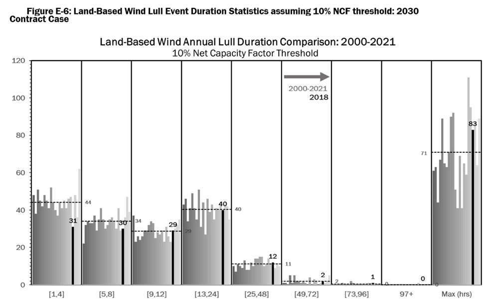
Figure E-6 presents the results of reviewing the LBW profiles over the 2000-2021 period on an annual basis assuming a 10% hourly NCF threshold (i.e., lull hours are defined as those with a NCF less than 0.1). The x-axis displays the event duration bins (e.g., “[1,4]” collect all one-to-four-hour events while “97+” collects all events that are 97 hours or longer) except for the last bin that displays the longest duration event in hours during the year. Each bar within a bin going from left to right represents the number of events in each duration bin for one year from 2000-2021, with 2018 labeled with black bars and the corresponding number of events. The dashed line across each bin shows the average value of the number of lulls (and maximum duration) across the 22-year period. The analysis shows that, in 2018, the longest event where LBW output stayed below 10% of capacity across New York was 83 hours long and there were 12 events between 25 and 48 hours long. The chart also shows that there were less short duration LBW lull events in 2018 relative to the 22-year average but that there were in general more lulls longer than one day in duration than in a typical year.

The Appendix also presents results for OSW:

Comparison of the DNV renewable production shapes shows that LBW has more and longer wind lulls than the OSW shapes. This is expected, in part, as OSW has higher average capacity factors as shown in the monthly-hourly analysis earlier in this section.

The combination of resource lulls is most useful for planning:

Combining the LBW, OSW, and UPV shapes on a capacity weighted basis and performing the same analysis results in less lulls of all durations because the diversity in timing of production from the different generation types has the effect removing or splitting longer lulls into more shorter events.

I modified Figure E-8 to highlight the worst-case duration of a combined lull as shown by the red line.  It appears that there was a 36 period when 90% of the OSW, LBW and UPV resources were unavailable.  Keep in mind that light winds are associated with high-pressure system weather that also correlates highly with extreme cold and hot temperatures that mean high electric loads.  This has resource planning ramifications that must also be addressed.

The Appendix concludes:

Analysis of the input renewable and load shapes over the course of a single year can provide significant information about when additional resources will most likely be needed to provide additional supply to the system. Using the 22-years of simulated renewable NCF profiles applied to the zonal capacity mix in the 2030 Contract Case provides significant insight into general system characteristics and potential needs for additional supply resources. Comparative review of these metrics for the 2035 Lower and Higher Demand scenarios in the Policy Case shows largely similar features across all of the discussed metrics but with larger impacts due to the higher loads and slightly larger renewable builds present in the 2035 Policy Case relative to the 2030 Contract Case.

Discussion

The NYISO has started to incorporate weather variability in future planning for an electric system that depends on wind and solar resources.  I want to make two points.

The current NYISO resource adequacy planning process is based on decades of experience with the existing system that relies on fossil, nuclear, and hydro resources.  Over the years, the resource planners have developed a good idea how much surplus capacity is needed on the system to ensure that when the load peaks that there will be adequate generation in place to service the load.  Those projections are based on the fact that outages across the system are not correlated for the most part.  These data show that there are frequent periods when all of the wind and solar resources are expected to provide much lower output than their rated capacity.  It appears that planners must account for a 36 hour period when all the LBW, OSW, and solar combined provide less than 10% of their rated capacity.  This is a huge challenge.

The second point is that the developing adequate resource to backup the wind and solar resources during these extended low resource periods must now account for weather variability.  These results are based on a 22-year data set and is analogous to the 100-year flood metric.  For flood management planning, analysts use the 100-year flood probability of a certain flood height to develop a resilient plan for the flood plain.  Future electric resource planning is going to have to develop something similar.  I am concerned that while the ramifications of a flood that exceeds the planning criteria are bad, the effects of inadequate electric power when New York has electrified homes, businesses, and transportation will be catastrophic.

I have long advocated a similar analysis that expands on this one.  Because New York depends on imports from adjoining regional transmission operators the geographical scope should be expanded to cover those regions.  The period of record should be as long as possible.  There are data available that could be used to extend the analysis to 1950.  Even if the resource planning is based on such a study, the over dependence upon weather related resources means that eventually there will be an even worse resource lull that causes a catastrophic blackout.  There is a limit to how much society can invest to avoid such an outcome, and I think that dynamic will inevitably lead to disaster. 

In addition, note that these results show that the Integration Analysis projections for future wind and solar capacity are underestimated.  The net capacity factors used are greater than the observed capacity factors.  This is another aspect of the state plan that needs to be reconciled with the most current NYISO work.

Conclusion

These results highlight the complications that weather-dependent electric grid planning must address.  Given the magnitude of the planning challenges I am not optimistic that planners will be able to anticipate all the effects to prevent reliability crises.  The results also destroy the myth that the wind and solar future grid will be more resilient than the existing grid.  That is just an empty slogan with no basis.